Fig. 1 a, b
T2-weighted (a) and postcontrast T1-weighted (b) 3D magnetic resonance urograms (MRU) show the anatomy and morphology of hydronephrotic and poorly functioning systems
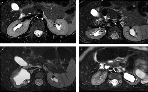
Fig. 2 a–d
High-resolution T2-weighted magnetic resonance urograms (MRU) of the kidney. The image a shows a patient with normal renal anatomy; the other three images are examples of patients with renal dysplasia. The high-resolution T2-weighted images can be used to assess renal parenchyma quality. Excellent corticomedullary differentiation allows assessment of both the renal cortex and medulla, as well as detection of cysts, scarring, edema, and architectural disorganization
Contrast Administration
One of the fundamental relationships that must be understood is the nonlinear relationship between signal intensity and GBCA concentration when using gradient-echo (GRE) imaging. At low concentrations, T1 effects predominate, and the relationship is relatively linear. However, as the concentration increases, T2* effects become increasingly important, leading to signal dephasing and an increasingly nonlinear relationship between signal and GBCA concentration. If the signal is to be used to estimate GBCA concentration, then it is important to keep the concentration low enough to ensure it is within linear range. If we want to operate in the nonlinear range, then a precontrast measurement of relaxation time is used to convert the measured signals to a concentration. In our implementation, hydration and furosemide injection, along with suitable pulse-sequence parameters, are used to keep the gadolinium signal within the linear range and hence allow the signal to be used as a measure of GBCA concentration.
We use the standard dose of a GBCA (Magnevist), as it provides excellent enhancement of the kidneys and allows evaluation of the MR nephrogram by differentiating the enhancing parenchyma from the background. Others use smaller doses of contrast, but we found the contrast to be inferior when using a lower dose, particularly when trying to segment poorly functioning kidneys. Because of the risks associated with using GBCA on patients in renal failure, a serum creatinine test is used on all patients to estimate glomerular filtration rate (GFR). If creatinine GFR is <60ml/min, we change the contrast agent to ProHance. To date, we have had no cases in which creatinine GFR was <30 ml/min, as patients with renal failure are not typically referred for an MRU. Caution should be used when using a GBCA, such as Eovist or MultiHance, which exhibit some degree of protein binding in order to enhance their relaxivity [10]. Whereas this enhances the aortic signal, similar binding will not occur in the tubular compartment unless proteinuria is present (and in this case, the degree of enhancement will depend on proteinuria concentration), thus negating the use of the arterial signal as the renal input function.
Initially we gave the contrast as a rapid bolus injection but found that the aortic signal intensity exceeded the linear portion of the curve and that the arterial signal was poorly characterized with the temporal resolution of 8–9 s typically used for our studies. Therefore, in order to obtain a well-characterized AIF that falls within the linear range, we now slowly inject the contrast agent using a power injector to control the infusion rate. We typically use a rate between 0.1 and 0.2 ml/s, and the injection usually takes between 20 and 60 s; we do not exceed a rate of 0.25 ml/s for small children.
Dynamic Contrast-Enhanced Imaging
As the GBCA is being injected, we acquire sequential dynamic 3D T1-weighted GRE sequences in the oblique coronal plane (Fig. 3). We typically use an acquisition time of 8–9 s per volume, using parallel imaging with a factor of 2. The flip angle is set at 30° in order to improve linearity of the signal intensity, and we use a high bandwidth to minimize TE. Our slice thickness is typically 2 mm, and we typically acquire 50 volume acquisitions in the first 10 min after contrast injection. We acquire continuous volumes for the first 5 min of scanning and then insert delays of increasing duration between the dynamics, as high temporal resolution is not required for the washout phase. An MIP image of each dynamic series is automatically generated, which facilitates a rapid review of data sets. We term this MIP image of each volumetric data set a concatenated MIP. Occasionally, if we want to outline the ureter and there is a fluid level within the renal pelvis, we turn the patients prone to promote drainage from the collecting system.
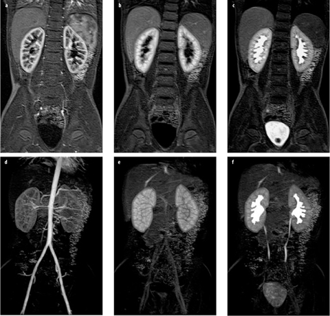
Fig. 3 a–f
Normal magnetic resonance urogram (MRU) in an 8-year-old girl. a–c The same slice from three volume acquisitions acquired at time points corresponding to cortical (arterial), parenchymal, and excretory phases of renal function, respectively. d–f Maximum intensity projections derived from the total volume for the same three time points
The dynamic data sets are reviewed to assess kidney perfusion, filtration, concentration, and excretion (Fig. 3). The aorta and renal arteries are usually well visualized on early dynamic images. This is helpful in identifying accessory arteries and crossing vessels associated with ureteropelvic junction (UPJ) obstruction [11]. The parenchymal phases are typically divided into cortical, medullary, and excretory phases. The cortical phase reflects both renal perfusion and glomerular filtration. The medullary phase typically occurs 45–90 s later and reflects perfusion of the renal medulla and concentration of the contrast agent in the loop of Henle. In the normal kidney, signal intensity in the renal medulla is always greater than in the cortex in this phase. After a further 30–60 s, contrast medium is excreted into the pelvicalyceal system and ureter in normal kidneys. Typ ically, signal intensity versus time curves are generated for the whole kidney but can be generated for specific tissues or regions of the kidney, if necessary (Fig. 4).
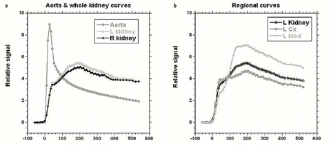
Fig. 4 a, b
Time intensity curves for patient shown in Fig. 3. These allow assessment and comparison of renal perfusion, concentration, and excretion similar to the time activity curves generated with diuretic renal scintigraphy. For this patient, volumetric differential renal function (vDRF) and Patlak (p)DRF were both 53:47 (L:R); unit Patlak per milliliter of tissue (up)DRF and tubular output (to)DRF were both 50:50
High-Spatial-Resolution Imaging
Once contrast is excreted into the ureters, we obtain high spatial resolution images in order to delineate optimally urinary tract anatomy. We are able to define the renal cortex, medulla, and pelvicalyceal system, as well as the course of the ureters to the bladder. These images are excellent for 3D VR either on the scanner or on an independent workstation (Fig. 1). For infants and small children, data is acquired using isotropic voxels 0.9 mm in size. In older children, we are limited to breath-hold imaging, which requires shorter imaging time and therefore decreased spatial resolution. In older children, we typically acquire voxels with a nominal spatial resolution of approx. 1.5 × 1.5 × 2.5 mm.
Postprocessing
The basic steps in postprocessing dynamic series are kidney segmentation, derivation of arterial and parenchymal curves, and fitting these to an appropriate model in order to derive indices of renal function. Segmentation provides both an estimate of renal volume, which is required when calculating GFR for the whole kidney, and a mask that determines the pixels contributing to the average time course for the kidney. We use a statistical approach in which the user selects a time point and outlines kidney location; then, statistical distribution of the signal in the selected dynamic (time point) and time-course information from each pixel are used to segment the kidneys [12]. The user then reviews the segmentation and if further refinement is required, then additional constraints can be added and the segmentation repeated until an acceptable segmentation is obtained. For most kidneys, little or no segmentation refinement is required, but for poorly functioning kidneys, achieving an acceptable segmentation can be quite time consuming. Rusinek et al. reported achieving good results with an algorithm based on the graph-cuts method [13]. Prior to fitting the signals for the kidney(s) and the AIF (see below) to a model, the signals must be converted into concentrations of contrast agent. This is usually done in one of two ways: (1) assuming a linear relationship between contrast agent concentration and signal change with respect to precontrast signal; (2) signal changes are converted, with the help of additional scans, to changes in T1, which can then be converted to changes in contrast agent concentration. The main disadvantage to method 1 is that it is only true for a restricted range of concentrations [14]; thus, a reduced dose of contrast and/or a slow injection protocol are required to limit the peak concentration of both AIF and kidneys, whereas hydration and the effect of furosemide provide additional reductions in renal concentration of contrast. The main advantage of this method is that it is simple to implement and does not require any additional images other than one or more precontrast images (which will generally be acquired anyway). Method 2 potentially offers greater precision and latitude in choosing contrast dose and injection protocol. However, this approach generally requires additional scans prior, and in some case after, the dynamic series, such that T1 values can be derived and then used to derive the equilibrium magnetization so T1 can be calculated for each dynamic volume [15]. Additionally, for clinical applications, time constraints will generally limit the amount of additional data that can be acquired, which in turn limits the precision of the T1 calculation. It should also be noted that the method also uses values for relaxivity of the contrast agent, which are typically derived from ex vivo experiments and may well not apply to the very different environment encountered in the kidney, where relaxivity value will vary between different tissues [16]. It should be noted that some models of renal function require a compact bolus of contrast, resulting in high first-pass concentrations of contrast, which hence require the use of the T1 conversion.
For our studies, we use method 1 in conjunction with a slow injection of contrast (minimum duration 20 s) and the use of hydration and furosemide to help restrict the maximum renal concentration. Baseline (precontrast) signal (S0) is averaged over the precontrast dynamics and the relative signal (change in signal) is calculated as [(S(t)−S0)/S0]. At a field strength of 1.5 T with our standard dynamic sequence, we found a linear relationship between relative signal and contrast agent up to concentrations of ∼1.5 mM in phantom studies [14].
Arterial Input Function (AIF)
In order to model renal function, an estimate of GBCA vascular concentration time course is required, and this is generally referred to as the AIF. The AIF is required, as vascular concentration affects GBCA filtration rate by the kidneys; even with a standardized dose and injection protocol, there will be idiosyncratic variations in AIF caused by physiological differences. For renal studies, the arterial signal is usually measured in a region of interest (ROI) in the descending aorta, the renal arteries being typically too small for reliable measurements in children. The aorta is viewed in both coronal and sagittal planes in order to minimize partial volume effects by excluding, if possible, regions where the aorta cuts through the imaging plane. The ROI consists of an arbitrary number of points — the points typically being positioned at or below the level of the renal arteries in order to minimize inflow effects. Even with careful selection of ROI location, pulsatility effects can still be present, and it is not always possible to eliminate partial volume and inflow effects. Imprecision in the AIF is one of the main factors that prohibit a reliable quantification of GFR with MRU. Several methods have been suggested to address this problem [17, 18], but none of these are yet close to routine clinical use. For methods based on the differential function then, AIF imperfections are common to both kidneys and hence are cancelled out [19].
In order to smooth out signal fluctuations and allow an estimate of the aortic signal at any given time point, the signal measured in the ROI is fitted to the model outlined below in order to generate a smooth AIF.
(1)
(2)
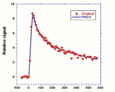
Fig. 5
Arterial input function. Measured data is shown by the dots, whereas the line is the best fit to Eqs. 1 and 2 using a nonlinear fitting procedure
The measured AIF is the whole blood AIF, but when the AIF is applied to models of renal function, plasma concentration is required, as GBCA is confined to plasma. Plasma concentration (C p ) is derived by correcting for hematocrit (Hct) using the formula given below:
(3)
Standard values for hematocrit are frequently assumed, but in young children, in whom hematocrit shows considerable variation with age, or in disease states in which hematocrit may be altered, using a standard value may lead to significant errors when trying to calculate an absolute GFR value.
Concentration versus Time Curvesc
Deriving the mean signal from the segmented volumes and converting the signal values to concentrations allows concentration versus time curves to be derived. Although the contrast dynamics can be assessed visually, the curves can provide extra information that is not always apparent from a visual inspection. Figure 4 shows both whole-kidney curves and segmental curves for the renal cortex and medulla (with the latter requiring additional segmentation). For all curves, the initial sharp increase in signal predominantly reflects the perfusion phase, with the renal cortex enhancing more than the medulla due to its higher blood volume. Because we use a slow injection of contrast, the vascular peak is less prominent than that seen when a compact bolus is used [24]. Following the vascular phase, a slight peak is seen in the cortical phase around 90 s after the initial arrival of contrast, and this represents GBCA arrival into proximal tubules. The main cortical peak, which occurs ∼100 s later, represents contrast in the distal tubules. As the GBCA passes through the loop of Henle, the peak signal for the medullary curve occurs prior to the main cortical peak. After the peaks in both curves, there is a general decline in signal intensity due to contrast excretion into the urine and the ongoing decline in GBCA plasma concentration.
Although it is possible to segment the cortex and medulla separately (Fig. 4), it is time consuming, and for this reason, we evaluate only whole kidney curves for the majority of cases. These curves are rapidly generated and enable assessment of perfusion, concentration, and excretion for each kidney and are analogous to the time activity curves of renal scintigraphy. These curves reflect the changes that occur in the renal parenchyma only, rather than in the parenchyma and collecting systems as seen with renal scintigraphy. As postprocessing becomes easier, segmental analysis will become more practical and provide greater insights into the anatomic and pathophysiologic changes occurring in the different compartments with various renal diseases. Similarly, fitting the models on a pixel-by-pixel basis to produce statistical parametric maps of the model parameters is yet too time consuming for routine clinical use, but as increased computational power becomes available, these will also become clinically feasible.
Modeling Renal Function
Several models of renal function have been developed and compared in the literature [3] and described in a review [25]. Therefore, we only briefly describe the specific techniques we use for clinical applications. The Rutland-Patlak model [26–28], which is widely used in single-photonemission computed tomography (SPECT) and CT has been applied to dynamic contrast-enhanced magnetic resonance imaging (DCE-MRI) data [1, 29]. With this model, GFR is measured as the transfer of GBCA from arterial blood to renal tubules, and the fact that the kidney includes both vascular and tubular components is taken into account. The amount of GBCA in any one kidney at a time point, C k (t), prior to GBCA excretion, can be expressed as the sum of the GBCA in the vascular space and nephrons. Assuming GBCA plasma concentration in the vascular space is proportional to plasma concentration in the aorta, C p (t), then defining the constants k 1 and k 2 to represent the vascular volume within the kidney and GBCA clearance from the vascular space, respectively, one can write
where t=0 is GBCA arrival time. The values for C p (t) and C k (t) are derived from the AIF and renal curves, respectively. Equation 4 can be rewritten in the form of a linear equation, and values for k 1 and k 2 derived from the plot of this equation. However, this requires choosing a start point (time when contrast agent is uniformly distributed in the vasculature) and an end point (excretion of contrast) for the plot, and it is simpler to apply a non linear fit of Eq. 4 to all data points between GBCA arrival and excretion in order to derive values for k 1 and k 2 [30].
(4)
Typically, one measures the average GBCA concentration within the kidney; thus, k 2 represents clearance per unit volume of tissue, which we refer to as the unit GFR. We believe this quantity is related to the singlenephron GFR and note that this quantity is reduced in decompensated, as well as dysplastic and uropathic, kidneys. An estimate of single-kidney GFR (SK-GFR) can be obtained by multiplying k 2 by renal volume (Vr). The Patlak model breaks down after a certain time because it fails to take account of the onward transport of GBCA (i.e., drop in signal seen at later time points in the parenchymal curves). Annet et al. developed a model that includes an additional term that accounts for the onward transport of GBCA and hence allows the whole time course to be modeled [2]. Their equation is of the form:
(5)
In their original article, Annet et al. confined their analysis to the renal cortex, and the term k ep represented the rate constant of GBCA transport out of the renal cortex and into the medulla. We apply the model to the whole kidney, and in this context, k ep is the rate constant of GBCA excretion from the kidney, which we refer to as the tubular output. A nonlinear fit of Eq. 5 can be applied to all points acquired after GBCA arrival, and hence, no preselection of the range of data points is required. In addition, Annet et al. modified C p by including a delay time (δ) to account for transit time from the arterial ROI to the renal parenchyma and a term to account for GBCA dispersion during this time. If only the delay term is incorporated, then C p (t) is replaced by a time-shifted plasma concentration C p (t-δ). Because the transit times are exponentially distributed [31], the dispersion term can be expressed as a convolution of the time-shifted plasma concentration with the mean transit time of the plasma compartment (MTT p ) [2, 32]. The plasma concentration corrected for delay and dispersion (C′ p ) is given by:
(6)
The vascular contribution is determined primarily by the aortic concentration scaled by the plasma fractional volume, and if dispersion is not accounted for, then an artificially low plasma volume is often derived in order to achieve the required scaling of the arterial concentration. This results in a vascular component with a low peak and a low “tail”, causing most of the rest of the renal curve to be attributed to glomerular filtration. When dispersion is accounted for, the vascular component is broader, with a more pronounced tail leading to less of the curve being attributed to glomerular filtration. Thus, accounting for dispersion is expected to result in more accurate GFR values. However, due to the less stable fitting caused by introducing the convolution and the extra terms (δ and MTTp) to the fitting process, combined with the limited temporal resolution used in our studies, we do not model dispersion, using a fixed delay instead.
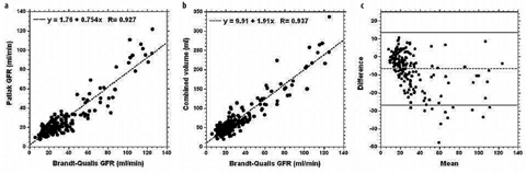
GFR Index
The majority of studies assessing the accuracy of the GFR estimates derived using MRU used measurements based on multiple blood samplings as the gold standard [1, 3]. However, such measurements are not routinely performed in a clinical setting (and only tend to be acquired for small numbers of volunteers in research studies). Absolute measurement of GFR is difficult, and the only clinical measure of GFR obtained on our patients is serum creatinine. There are several well-known shortcomings of this method, but when combined with suitable corrections, a reasonable estimate of GFR can be obtained [33]. Figure 6 shows the results of comparing total GFR as estimated from serum creatinine using the Brandt-Qualls formula, with the combined (i.e., sum of both kidneys) Patlak slope of the two kidneys for 195 patients. As hematocrit was not measured for these patients, no hematocrit correction (Eq. 3) was performed. For the correlation plot, the relationship can be seen to be linear to a good approximation, but with the Patlak values being lower than the Brandt- Qualls values. The Bland-Altman plot shows both offset (−6.6 ml/min) due to GFR underestimation by the Patlak techniques, and the 95% confidence intervals (CI) (±10.1 ml/min). Because of these fairly wide confidence limits and the presence of a number of outliers, it seems reasonable to use the functional measurements as an index, rather than an absolute measure, of GFR. We and others [30] found that the linear and nonlinear Patlak techniques produce similar GFR index values. We prefer to use the nonlinear technique, as it requires choosing only an end time point, rather than start and end time points, and it uses more points. The Annet model produces systematically higher values for the GFR index in our implementation. Figure 6 also shows that there is a reasonable correlation between total renal volume (i.e., sum of the volume of both kidneys) and GFR.
 Enterography: Small Bowel Imaging That Impacts Patient Management
 to Perform and Report Magnetic Resonance Imaging for Pelvic Floor Dysfunction: An Interactive Case-Based Approach
 Should it Be Integrated into Screening and Clinical Routine Imaging?
 Vascular Disease: Diagnosis and Therapy
 and Acquired Pathologies of the Pediatric Gastrointestinal Tract
 for the Spread of Disease in the Abdomen and Pelvis


Related posts:
Enterography: Small Bowel Imaging That Impacts Patient Management
to Perform and Report Magnetic Resonance Imaging for Pelvic Floor Dysfunction: An Interactive Case-Based Approach
Should it Be Integrated into Screening and Clinical Routine Imaging?
Vascular Disease: Diagnosis and Therapy
and Acquired Pathologies of the Pediatric Gastrointestinal Tract
for the Spread of Disease in the Abdomen and Pelvis
Stay updated, free articles. Join our Telegram channel
Full access? Get Clinical Tree
