Level of Measurement

The level of measurement (or measurement scale) of a variable is its designation as continuous or discrete. A continuous variable has values taken, at least theoretically, from a continuum of the real number line. Examples are gestational age, BP, and BMI. A discrete variable has discrete values (i.e., values not coming from a continuum of the real number line). Examples are gender (male, female), severity of disease (low, medium, high), and type of operation (standard, modified, laparoscopic). The “severity of disease” variable is called an ordinal discrete variable because there is an order associated with its levels; the “type of operation” variable is called a nominal discrete variable because there is no order associated with its levels.

Variable Structure

A dependent variable (also called outcome, endpoint, or response variable) is the primary variable of a research study. It is the behavior of such a variable that is of primary concern, including the effects (or influence) of other variables on it. An independent variable (also called explanatory, regressor, or predictor variable) is the variable whose effect on the dependent variable is being studied. Designation of which variables are dependent and which are independent in a research study establishes the variable structure. How a variable is handled statistically depends in large part on its level of measurement and its variable structure.¹

Completely Randomized Design (CRD)

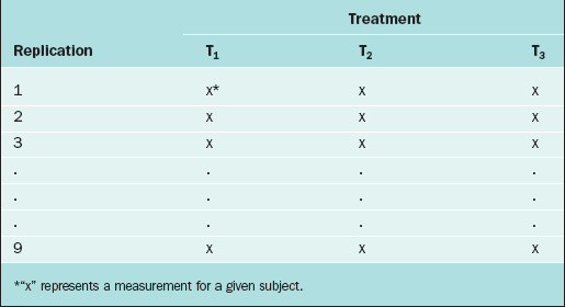
In the CRD, subjects are randomly assigned to experimental groups. As an example, suppose that the thickness of the endometrium is observed via ultrasound for women randomly assigned to three different fertility treatments (treatments T₁, T₂, and T₃). Twenty-seven subjects are available for study, so 9 subjects are randomly selected to receive treatment T₁, 9 are randomly selected from the remaining 18 to receive treatment T₂, and the remaining 9 receive treatment T₃. The data layout appears in Table 9-1.

Table 9-1 Data Layout For a Completely Randomized Design

In addition to randomness, an important assumption of the CRD is that the samples are independent (i.e., the outcome measurement—in this case, endometrial thickness—for one subject is not related to that of any other subject). For instance, two related subjects (e.g., sisters) should not both be included in the data set because they are genetically related and hence their endometrial thicknesses may be correlated.

The principles of the CRD are the same for a survey, where subjects form groups in a natural way. For instance, in comparing the mean cholesterol level among first-, second-, and third-trimester pregnant women, a random sample of all pregnant women can be obtained, and then each woman can be naturally classified as being in the first, second, or third trimester. In this case, the sample size for each group will likely not be the same. Alternatively, random samples of 10 first-trimester, 10 second-trimester, and 10 third-trimester women can be obtained (stratified sampling).

Note in these examples that the principles of randomization and replication are used. The following design is used for controlling or blocking.

Randomized Complete Block Design (RCBD)

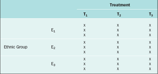
The RCBD is a generalization of the CRD whereby a second factor is included in the design so that the comparison of the levels of the treatment factor can be adjusted for its effects. For example, in the endometrial thickness study, there may be three different ethnic groups of women, E₁, E₂, and E₃, included in the study. Because the variation of the endometrial thicknesses may be higher between two different ethnic groups than within a given ethnic group, it would be wise to block on the ethnic group factor. In this case, we would randomly select 9 subjects from ethnic group E₁ and randomly assign 3 to each of the three treatments; likewise for ethnic groups E₂ and E₃, for a total of 27 subjects. The data layout would appear as in Table 9-2.

Table 9-2 Data Layout For a Randomized Complete Block Design

Latin Square Design (LSD)

To control for a second factor, a Latin square design is used. For example, the subjects in the endometrial thickness study come from three different age groups, A₁, A₂, and A₃. Because the endometrial thickness variable is likely to be more homogeneous for subjects from a given age group than for subjects from two different age groups, we should block on the age group in addition to the ethnic group.

Repeated Measures Design

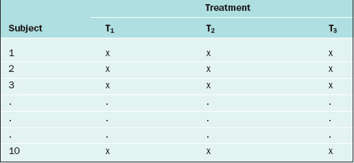
If in the RCBD the blocking factor is the subject, and the same subject is measured repeatedly, then the design becomes a repeated measures design. For instance, suppose that each of 10 subjects receives three different BP medications at different time points. For each medication, the BP is measured 5 days after the medication is started, then there is a 2-week “wash-out period” before starting the next medication. Also, the order of the medications is randomized. The data layout appears as in Table 9-3.

Table 9-3 Data Layout For a Repeated Measures Design

Many more sophisticated and complex experimental designs exist, and can be found in any standard text on experimental design.^4,5 For evaluating the validity, importance, and relevance of clinical trial results, see the article by The Practice Committee of the American Society for Reproductive Medicine.⁶ For surveys, there are many ways in which the sampling can be carried out (e.g., simple random sampling, stratified random sampling, cluster sampling, systematic sampling, or sequential sampling).^7,8

Continuous Variables

The principal descriptive features of continuous variables are (1) central location and (2) variability (or dispersion).

An important numerical measure of the centrality of a continuous variable is the mean:

Alternative measures of centrality are the median (middle measurement, or average of the two middle measurements if n is even, in the list of measurements rank-ordered from smallest to largest) and the mode (most frequent measurement).

A simple numerical measure of the variability or dispersion of a continuous variable is the range: the largest measurement minus the smallest measurement. The larger the variability in the measurements, the larger the range will be. A more common numerical measure of variability is the variance:

Note that the variance is approximately the average of the squared deviations (or distances) between each measurement and its mean. The more dispersed the measurements are, the larger s² is. Because s² is measured in the square of the units of the actual measurements, sometimes the standard deviation is used as the preferred measure of variability:

Also of interest for a continuous variable is its distribution (i.e., a representation of the frequency of each measurement or intervals of measurements). There are many forms for the graphical display of the distribution of a continuous variable, such as a stem-and-leaf plot, boxplot, or bar chart. From such a display, the central location, dispersion, and indication of “rare” measurements (low frequency) and “common” measurements (high frequency) can be identified visually.²

It is often of interest to know if two continuous variables are linearly related to one another. The Pearson correlation coefficient, r, is used to determine this. The values of r range from –1 to +1. If r is close to –1, then the two variables have a strong negative correlation (i.e., as the value of one variable goes up, the value of the other tends to go down [consider “number of years in practice after residency” and “risk of errors in surgery”]). If r is close to +1, then the two variables are positively correlated (e.g., “fetal humeral soft tissue thickness” and “gestational age”). If r is close to zero, then the two variables are not linearly related. One set of guidelines for interpreting r in medical studies is: |r| > 0.5 ⇒ “strong linear relationship,” 0.3< |r| ≤ 0.5⇒ “moderate linear relationship,” 0.1 < |r| ≤ 0.3⇒ “weak linear relationship,” and |r| ≤ 0.1⇒ “no linear relationship”.^9,10

Discrete Variables

For summarization of a discrete variable, a frequency table is used: for each discrete value of the variable, its frequency (how many times it occurs in the sample of, say, n observations) and relative frequency (frequency/n) are recorded. Of course, the sum of the frequencies over all of the discrete levels of the variable must be n, and the sum of the relative frequencies must be 1.0 (100%).

For two discrete variables the data are summarized in a contingency table. A two-way contingency table is a cross-classification of subjects according to the levels of each of the two discrete variables. An example of a contingency table is given in Table 9-4.

Table 9-4 Contingency Table for the Cross-classification of Subjects According to Treatment and Outcome.

Here, there are a + b + c + d subjects in the sample; there are “a” subjects under the standard treatment who died, “b” subjects under the standard treatment who survived, and so on. If it is desired to know if two discrete variables are associated with one another, then a measure of association must be used. Which measure of association would be appropriate for a given situation depends on whether the variables are nominal or ordinal or a mixture.^11,12

In medical research, two of the important measures that characterize the relationship between two discrete variables are the risk ratio and the odds ratio. The risk of an event, p, is simply the probability or likelihood that the event occurs. The odds of an event is defined as p/(1–p) and is an alternative measure of how often an event occurs. The risk ratio (sometimes called relative risk) and odds ratio are simply ratios of the risks and odds, respectively, of an event for two different conditions. In terms of the contingency table given in Table 9-4, these terms are defined as follows.

Note that a risk ratio of 4.0 means that the risk of death under the standard treatment is four times that under the new treatment. An odds ratio of 4.0 means that the odds of death are four times higher under the standard treatment than under the new treatment.

Another important measure in clinical practice is the risk difference, RD, the absolute difference between the risk of death under the standard treatment and the risk of death under the new treatment:

The inverse of the risk difference is the number needed to treat, NNT:

For example, in a study by Marcoux and colleagues¹³ 341 women with endometriosis-associated subfertility were randomized into two groups, laparoscopic ablation and laparoscopy alone. The study outcome was “pregnancy > 20 weeks’ gestation.” Of the 172 women in the first group, 50 became pregnant; of the 169 women in the second group, 29 became pregnant (a = 50, b = 122, c = 29, and d = 140). The risk of pregnancy is 0.291 in the first group and 0.172 in the second group; the corresponding odds of pregnancy are 0.410 and 0.207. The risk ratio is 1.69 and the odds ratio is 1.98. The likelihood of pregnancy is 69% higher after ablation than after laparoscopy alone; the odds of pregnancy are about doubled after ablation compared to laparoscopy alone. The risk difference is