(1)
Department of Vascular Surgery, Evangelisches Krankenhaus Königin Elisabeth Herzberge, Berlin, Germany
The mechanics of solid bodies is fundamentally different from the mechanics of liquids and gases. The latter is called fluid mechanics. Flowing gases and liquids are summarized as fluids (Prandtl et al. 1990; Tipler and Mosca 2009). An accurate definition of the word fluid involves motion: “Fluid is free to change in form” (Munson et al. 1994).
Hemodynamics deals with the physical basics of blood flow. As opposed to other real flows, blood flow is characterized by its pulsatility and its flow-dependent viscosity.
20.1 Principles of Fluid Mechanics
For the description of some essential laws of fluid mechanics, the understanding of the following terms is necessary:
Stationary and non-stationary flow
Streamline, pathline, and streakline
Stagnation point
Reynolds number, laminar and turbulent flow
Dead water zone
If the flow is not time dependent, it is called stationary. Then the same unchanging flow pattern may be found at any moment in time. Conversely, a time-dependent flow with continuously changing flow patterns is called non-stationary. Therefore the pulsatile flow in the blood circulation is non-stationary.
Flow velocity denotes the change of position per time unit. It is a vector. Therefore it needs a magnitude, a direction, and a starting point (e.g., the coordinates of a fluid particle). A single vector characterizes the velocity of a single point mass (an infinitely small fluid particle). If the starting points of the vectors of a flow pattern are connected in such a way that the vectors become curve tangents, the resulting lines are called streamlines. Streamlines help illustrate flow patterns (cf. Fig. 4.17). They do not kink, and they do not intersect. At a given point there cannot be two velocities at the same time (Bohl 1994; Prandtl et al. 1990). Zero velocity streamlines at the stagnation point constitute an exception (see below), as they may intersect and branch out. Imagine numerous swimming tea lights on a water surface. If you took a photo after an exposure time which is just long enough to change the light points into lines, they would be streamlines.
With stationary flows, streamlines are the same as pathlines. With nonstationary flows, however, this is not the case: Streamlines depict the momentarily simultaneously existing velocity directions, whereas pathlines show the velocity directions of a particle over a course of time. In our thought experiment with the tea lights, you would have to have a very long exposure time in order to obtain the pathline of a single tea light.
Streaklines are a third type of lines. They are the curves of all particles that pass the very same topographical point over the course of time. In an experiment streaklines may be visualized by injecting dye at a certain point (in the thought experiment: a chain of tea lights) (Smits and Lim 2000). Then all particles which pass this point will be colored (e.g., Fig. 4.5). If you place a static solid body into a flow, the streamline that meets the body will divide according to the solid body’s shape and flow around it. The front branch point is called stagnation point.
At this point the whole kinetic energy of the fluid is completely transformed into pressure, and the flow comes to a standstill (Gersten 1991; Prandtl et al. 1990). The pressure at the stagnation point is called stagnation pressure (cf. Bernoulli’s law, Chap. 20.2). Likewise you can also find stagnation points when the flow hits a wall (cf. Fig. 4.9a).
In order to compare flows in geometrically similar structures, dimensionless quantities are used. The most important is named after Osborne Reynolds (1842–1912). For the flow in pipes it is
 with
with  – mean velocity, d – diameter of the pipe, ρ – density, and η – dynamic viscosity.
– mean velocity, d – diameter of the pipe, ρ – density, and η – dynamic viscosity.A laminar flow is a stratified flow. Between neighboring layers there is no exchange of fluid particles perpendicular to the flow direction. A laminar flow of a real fluid in a pipe (blood vessel) has a parabolic velocity profile (Fig. 20.1). The velocity reaches its maximum in the center of the pipe and drops to zero at the walls (no slip condition, cf. Chap. 20.4); the change from a laminar flow into a turbulent flow occurs at the critical Reynolds number of Re = 2,300 (Gersten 1991; Opitz and Pfeiffer 1984; Zamir 2000). Other authors do not see such a strict cut off. Below Re = 2,000 there is a laminar flow, and above Re = 3,000 the flow is turbulent. In between, the flow pattern is unstable and can swing from one state to the other (Tipler and Mosca 2009). The turbulent flow is characterized by random oscillations which are superimposed upon the basic flow. There is an intensive exchange of fluid particles between the different layers, which mix even more with increasing Reynolds numbers. The velocity profile flattens in the center of the tube, and is almost evened out with high Reynolds numbers. Apart from the zones near the wall, it is almost constant over the entire cross section. Except for the conditions at systolic peak velocity in the ascending aorta, the in vivo Reynolds numbers in the human circulation are below the critical region (Opitz and Pfeiffer 1984; Prandtl et al. 1990).
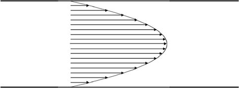
Fig. 20.1
Parabolic velocity profile of the laminar flow in a pipe
During an experiment, Reynolds directed a thin line of dye into a flow. With a laminar flow the dye stays together within a thin compact fluctuating line. In a turbulent flow the line dissolves quickly over the whole cross section.
A dead water zone is not or hardly perfused. Such regions develop behind the regions of flow separation (cf. Chap. 20.3). The basic flow is significantly slowed. Depending on the Reynolds number, regular vortices or a turbulent flow form. The dead water region is separated from the laminar main stream by a divisive line. In the dead water zone the flow is much less harmonious than in the main stream and can stagnate completely under extreme conditions (e.g., in certain regions behind a closed mechanical heart valve). In the dead water zone there are especially long interactions between the flow and the vascular wall. These regions are predestined for thrombus formation or the lining of the wall with “pseudointima” (cf. Chap. 4.1, Heise et al. 2011).
20.2 Continuity Equation
If you determine the velocities of the particles which flow through an arbitrary area A, then the average of these velocities can help establish the volume of the flow that passes the area A during the time interval Δt:
The division of both sides of this equation by Δt yields the volume over time, the volume flow, which is most often referred to as flow rate or simply flow Q. In medicine the common measuring unit is Q = [mL/min].
With flowing incompressible fluids without air or other gas inclusions in an impermeable pipe, it seems obvious that the same amount of fluid which enters the pipe during a given interval of time must also leave the pipe during the same time. Fluid is neither added nor lost. If the cross section is constant, then
This equation is called the continuity equation and describes the conservation of mass. Transferred to a vessel with changing cross sections (Fig. 20.2a) this means that the flow rate in the different areas A1 and A2 is constant. If the cross section changes, the mean flow velocity also has to change. Further considerations can be found in Chap. 20.4.
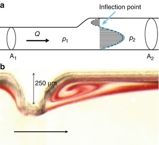
Fig. 20.2
(a) As the pipe diameter increases, there will be flow separation. The mark shows the inflection point of the velocity profile (zero velocity). (b) Further downstream a vortex will form (microscopic photo of a reproduced vascular wall in the pulsatile flow model; the arrow indicates the flow direction)
20.3 Bernoulli’s Equation
In a stagnant fluid the pressure which a fluid column exerts on its base depends on its height:
 with p – hydrostatic pressure, ρ – density, g – gravity, and h – height.
The pressure is the same for all points of a certain height (constant over the whole cross section) and increases proportionally with height.
A pressure p 0 which is exerted on the surface of a non-flowing fluid (e.g., via a piston) leads to a uniform increase in pressure everywhere in the fluid (Pascal’s principle). Then the total pressure p G is
With flowing fluids, an additional pressure component has to be taken into account: the dynamic pressure or stagnation pressure. It depends on the velocity v:

Example: Dynamic Pressure on the Floor of the Venous Anastomosis
The density of the model fluid is ρ = 1.1 g/cm3 (Chap. 4.2). Figure 4.11a shows the approximate velocity at the stagnation point: v = 0.75 m/s. Supposing that the flow hits the venous wall at this speed (conversion factors 1 N = 1 kg × m/s2 and 1 Pa = 1 N/m2), the resulting dynamic pressure is
The pressure maximum in Fig. 4.13 is 322 Pa. The accordance is quite good considering that, at a supposed velocity of 0.77 m/s, the calculated dynamic pressure is 326 Pa.
To estimate this value the pressure is converted into mmHg: p = 322 Pa = 2.4 mmHg. At the venous anastomosis the pressure decreases by 10 mmHg (Fig. 4.13a, b). This means that at the stagnation point the pulsatile stress is 24 % higher than in the other anastomotic regions.
The pressure equation of the Swiss mathematician and physicist Daniel Bernoulli (1700–1782) is a basic equation of fluid mechanics. It says that the combination of pressure, geodesic height, and flow velocity assumes the same value for each point of the flowline. The equation is also fundamentally important to the fluid mechanics of stationary, incompressible, and non-viscous flows. Its integrated form is
With incompressible flow pressure does not result in the compaction of the fluid but in a change in its motion. There is no internal friction in non-viscous fluids.
Related posts:


Stay updated, free articles. Join our Telegram channel

Full access? Get Clinical Tree


