Basic Magnetic Resonance Imaging Principles for the Abdomen and Pelvis
A basic understanding of a limited number of physical principles is essential to performing and interpreting abdominal and pelvic magnetic resonance imaging (MRI) examinations. However, it is not necessary, or even advisable, for most radiologists to understand MRI physics at the quantum level to perform high-quality clinical MRI studies. Few of us fully understand Einstein’s general theory of relativity, but none of us would willingly vacate an airplane at 15,000 feet without a parachute. In other words, a full understanding of the physics or mathematics of gravity is unnecessary to predict the behavior of an object within a gravitational field. Similarly, an in-depth understanding of MR physics remains a luxury for most radiologists, most of whom need more practical knowledge. Therefore, this discussion on abdominal and pelvic MRI is focused on the principles that are most relevant to the needs of practicing radiologists.
Disclaimer: Most of the discussions of MR physics in this text are based on Newtonian approximations. An understanding of the behavior of individual protons requires knowledge of quantum mechanics beyond the normal scope of working knowledge of most practicing radiologists. However, because MRI measures the signal of large populations of protons rather than individual protons themselves, these approximations are sufficient to predict behavior, which is really what interests clinical imagers. Attempts to explain all MRI phenomena using only Newtonian models may eventually result in frustration and confusion. Therefore, our simplistic explanations should be viewed not so much as statements of ultimate truth but rather as practical mnemonic devices beneficial to the clinical application of MR.
T1 and T2
Most abdominal and pelvic MR images fall into one of two categories: T1-weighted or T2-weighted. Differences in T1 relaxation times between tissues determine the image contrast in a T1-weighted image, and differences in T2 relaxation times between tissues determine the image contrast in a T2-weighted image. MR images are referred to as weighted, because no image represents only differences in T1 or T2 relaxation times. There is always some T2 contrast in a T1-weighted image and some T1 contrast in a T2-weighted image. Figure 1.1 illustrates the differences between these two types of images.
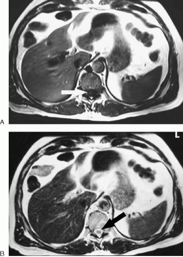 FIG. 1.1. T1-weighted image versus T2-weighted image. A: Axial T1-weighted spin echo image. Bright fat and dark fluid (cerebrospinal fluid [CSF]) (arrow) are characteristic of T1-weighted images. Signal intensity of liver is normally slightly greater than that of spleen. B: Axial T2-weighted fast spin echo image. Bright fluid (CSF) (arrow) is characteristic of T2-weighted images. Fat is also bright on fast spin echo images. Signal intensity of spleen is normally slightly greater than that of liver, a difference that is considerably more apparent on fat-suppressed images. |
The source of the signal measured by MRI is the hydrogen nucleus or proton. To understand T1 and T2, it is helpful to imagine what happens to these protons when placed in a magnetic field and exposed to radiofrequency (RF) pulses. Because protons may be thought of as spinning charged particles, they are associated with a small magnetic field (magnetic dipole moment). This magnetic field may be represented as a vector along the axis of the spinning proton. Normally, the magnetic field vectors of all of the body’s protons are randomly aligned. When placed in a strong external magnetic field (such as an MRI scanner), these vectors align parallel or antiparallel to the main magnetic field. Because slightly more proton vectors align in the parallel direction than the antiparallel direction, a net magnetization vector results, representing the sum of all the individual magnetization vectors of the protons. This net magnetization vector is referred to as longitudinal magnetization. The net magnetization vector is the one of interest.
The individual magnetic field vectors of protons placed in the MRI scanner do not actually align perfectly with the external field. Instead, they precess about the external magnetic field vector much like the earth precesses in space or a top precesses under the influence of gravity. In addition, the individual protons precess out-of-phase with one another much like a random assortment of spinning tops would be tilted slightly in different directions at any moment in time. Even though a group of hydrogen protons placed in an external magnetic field does not initially spin in-phase, protons
existing in a similar chemical environment precess at the same frequency according to the Larmor equation:
existing in a similar chemical environment precess at the same frequency according to the Larmor equation:
Resonant frequency (MHz) = [42.6 MHz/tesla][magnetic field strength (in tesla)]
The Larmor equation indicates that the precessional frequency of protons is directly proportional to the strength of the external magnetic field. In other words, hydrogen protons precess slower at 0.5 T than they do at 1.5 T. This has important implications for how signal from protons is localized in space and for techniques such as fat suppression.
To generate signal from protons placed within a magnet, two things must be accomplished. First, the protons must be made to precess in-phase (i.e., their magnetic field vectors point in the same direction) to yield maximal signal. Second, the net magnetic field vector must be tipped from the longitudinal axis (aligned with the external magnetic field) into the transverse plane (aligned perpendicular to the external magnetic field). This latter condition results from the need to create an oscillating magnetic field in the patient, which generates a current (the echo) in the receiver coil. These two conditions (creation of transverse magnetization and phase coherence) are accomplished with the application of an RF pulse at the resonant frequency of hydrogen protons.
The application of the RF pulse (which is actually an oscillating magnetic field) causes the longitudinal magnetization vector to spiral down into the transverse plane so it can be measured. This initial RF pulse is commonly referred to as an excitation pulse. The amount of transverse magnetization created depends on the amplitude and duration of the RF pulse. The angle between the original longitudinal magnetization and the new net magnetization vector created by the RF pulse is referred to as the flip angle.
Once the RF pulse is shut off, the protons begin to realign themselves with the external magnetic field. As this occurs, the net longitudinal magnetization vector regrows in a logarithmic fashion. The time it takes for approximately two thirds (63%) of the original longitudinal magnetization to regrow is referred to as the T1 relaxation time (longitudinal relaxation time) (Fig. 1.2). As longitudinal magnetization regrows, transverse magnetization diminishes (decays). This loss of transverse magnetization (an exponential decay function) not only results from the conversion of transverse magnetization back into longitudinal magnetization, but also from an energy exchange between protons (referred to as spin-spin interaction). The loss of transverse magnetization resulting from the interaction between hydrogen nuclei is an irreversible process. The time it takes for transverse magnetization to decay to approximately one third (37%) of its maximum value (as a result of irreversible causes) is referred to as the T2 relaxation time (Fig. 1.3).
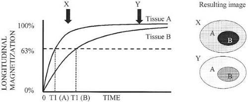 FIG. 1.2. T1 relaxation and T1 contrast. At time = 0, tissue A and tissue B are subjected to a 90 degree RF pulse, eliminating longitudinal magnetization. Tissue A recovers its longitudinal magnetization quicker than tissue B and, therefore, has shorter T1 relaxation time (when it recovers approximately 63% of its initial longitudinal magnetization). At time X (arrow X), there is a relatively large difference in longitudinal magnetization between tissue A and tissue B. Therefore, an image based on this difference (upper oval to right of graph) would have excellent T1 contrast. An image based on the difference in longitudinal magnetization at time Y (arrow Y) would have considerably less image contrast (lower oval to right of graph). |
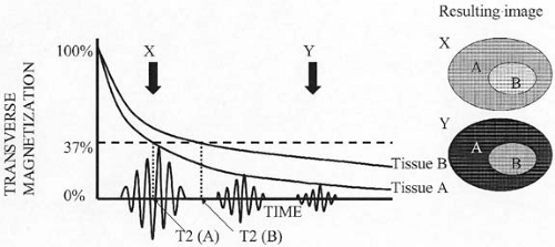 FIG. 1.3. T2 relaxation and T2 contrast. At time = 0, tissue A and tissue B are subjected to a 90 degree RF pulse, creating transverse magnetization. This excitation pulse is followed by three 180 degree refocusing pulses that result in three echoes (wavy lines). Only echoes for tissue A are shown on the diagram. The T2 relaxation curve follows echo peaks. Note that tissue A loses its transverse magnetization more rapidly than tissue B and, therefore, has shorter T2 relaxation time (when it decays to approximately 37% of its initial value). At time X (arrow X), there is a relatively small difference in transverse magnetization between tissue A and tissue B. Therefore, an image based on this difference (upper oval to right of graph) would have poor T2 contrast. An image based on the difference in transverse magnetization at time Y (arrow Y) would have considerably more image contrast (lower oval to right of graph). |
In a perfect world, the discussion of T1 and T2 would end here; however, no magnetic field is perfect. Subtle differences in the local magnetic field strength around individual protons are caused by imperfections in the scanner itself or the material (e.g., metal, air, tissue) placed within the scanner. This magnetic field heterogeneity increases the rate of loss of transverse magnetization. This occurs because protons precess at slightly different rates when exposed to slightly different local magnetic field strengths. Therefore, decay of transverse magnetization occurs more rapidly than would be predicted based on a perfect magnetic field. Unlike spin-spin interactions, loss of transverse magnetization resulting from static variations in local magnetic field strength is a reversible process. This more rapid loss and decay of transverse magnetization is referred to as T2*. In other words, T2* reflects
loss of transverse magnetization from both reversible (due to static magnetic field heterogeneity) and irreversible (due to spin-spin relaxation) causes. T2* is always shorter than T2, and T2 is always shorter than T1.
loss of transverse magnetization from both reversible (due to static magnetic field heterogeneity) and irreversible (due to spin-spin relaxation) causes. T2* is always shorter than T2, and T2 is always shorter than T1.
Different tissues in the body have different T1 and T2 values. For example, water has relatively long T1 and T2 values, whereas the T1 and T2 values of fat are considerably shorter. A tissue with a short T1 recovers full longitudinal magnetization faster than a tissue with a long T1, and therefore appears relatively brighter on a sequence designed to bring out the differences in T1 relaxation (a T1-weighted scan). A tissue with a short T2 loses transverse magnetization quicker than a tissue with a long T2, and therefore appears relatively darker on a sequence designed to bring out differences in T2 relaxation (a T2-weighted scan). These differences in T1 and T2 values give rise to most of the tissue contrast seen in abdominal and pelvic MRI.
Spin Echo Versus Gradient Echo
One of the major components of the MRI pulse sequence is the RF excitation pulse, which is used to convert net longitudinal magnetization into net transverse magnetization. For a spin echo sequence, this pulse is 90 degrees, which means that all of the initial longitudinal magnetization is converted into transverse magnetization. However, the initial net transverse magnetization decays too rapidly to be of much use in generating an image. This is because the transverse magnetization vectors of the individual protons rapidly lose their phase coherence (they become out-of-phase with each other
due to variations in the local magnetic field), resulting in loss of net magnetization. This initial rapid loss of signal is referred to as free induction decay, represented by T2*. To obtain a signal from which an MR image can be made, either RF refocusing or gradient refocusing must be done to bring the individual transverse magnetization vectors back into phase.
due to variations in the local magnetic field), resulting in loss of net magnetization. This initial rapid loss of signal is referred to as free induction decay, represented by T2*. To obtain a signal from which an MR image can be made, either RF refocusing or gradient refocusing must be done to bring the individual transverse magnetization vectors back into phase.
The spin echo family of pulse sequences makes use of a 180-degree RF pulse to bring the protons back into phase to create the echo, a process known as RF refocusing. The effect of the 180-degree pulse is to flip the individual transverse magnetization vectors so that the more rapidly precessing protons catch up with the slower protons, much like runners of different speeds realigning after their direction is reversed. The process of creating a spin echo is illustrated in Figure 1.4. A refocusing pulse of less than 180-degrees creates an echo, but a 180-degree pulse gives the maximum signal.
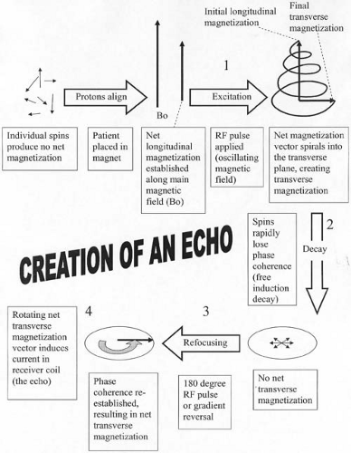 FIG. 1.4. Creation of a spin echo. Critical events in generation of an echo in MRI are (a) establishing longitudinal magnetization, (b) creating transverse magnetization through RF excitation, (c) decay of net transverse magnetization (loss of phase coherence), (d) refocusing of transverse magnetization (reestablishment of phase coherence), and (e) measurement of echo (induction of current in receiver coil). Large numbers correspond to time points in Figure 1.6, which are notated by the same numbers. |
Because a 180-degree pulse results in the strongest echo, one might think that it is always desirable to use this type of RF refocusing pulse. For a simple spin echo sequence, this is generally true. However, a 180-degree RF pulse is also associated with higher energy deposition in the patient (manifested as tissue heating) than a pulse with a lower flip angle*, because the higher flip angle requires increased amplitude or duration of the RF pulse. The use of a large number of 180-degree refocusing pulses (as may occur with fast spin echo or turbo spin echo imaging) can result in unacceptably high levels of energy deposition in the body, particularly if the RF pulses are spaced closely together. One way to prevent tissue heating and conform to Food and Drug Administration regulations is to reduce the refocusing pulses to less than 180-degrees (generally 150-degrees suffices).
In contrast to the spin echo family of sequences, gradient echo sequences make use of a gradient reversal to bring the protons back into phase to create the echo. In MRI, gradients are linear variations in magnetic field strength that are momentarily applied at specific times during a pulse sequence. A gradient applied along one axis of the body causes the protons along that gradient to precess at different frequencies according to the Larmor equation. Protons exposed to higher field strengths precess at a higher frequency than protons exposed to lower field strengths. The result of these different precessional frequencies is that the protons begin to dephase. By reversing this gradient, the protons can be made to rephase. One important difference between gradient refocusing and RF refocusing is that the former technique only corrects for dephasing induced by the initial gradient, whereas the latter technique also corrects for the effects of local magnetic field heterogeneities. Therefore, gradient echo pulse sequences are more susceptible to artifacts created by substances that alter the local magnetic environment of the proton, such as metal or air. Gradient echo sequences are preferred for the detection of iron (e.g., hemachromatosis) and spin echo sequences are preferred in the setting of implanted metallic prostheses. The initial RF excitation pulse is often less than 90 degrees for a gradient echo sequence, but any flip angle up to 90 degrees may be used. Examples of spin echo and gradient echo images are shown in Figure 1.5.
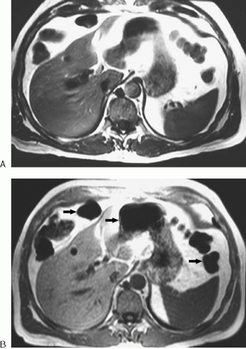 FIG. 1.5. Spin echo versus gradient echo. A: This axial spin echo T1-weighted image is the same as in Figure 1.1A. Acquisition time was approximately 2 minutes for the complete liver. Respiratory motion artifact was reduced by placement of a saturation band over anterior abdominal fat. B: Axial gradient echo T1-weighted image of the same patient. The entire liver was imaged in less than 30 seconds during breath-hold. The image has increased noise and more susceptibility artifact around bowel (arrows) than does the spin echo image. |
Repetition Time and Echo Time
Two of the most frequently altered MRI parameters are the repetition time (TR) and the echo time (TE) (Fig. 1.6). To spatially encode MRI data, the tissue protons must undergo a series of steps referred to as phase-encoding. For most MRI sequences, the initial RF excitation pulse and the refocusing pulse (in the case of spin echo) or gradient reversal (in the case of gradient echo) must be repeated many times. Each time this series of events is repeated, a different strength gradient (referred to as the phase-encoding gradient) is applied
to impart a phase difference upon the protons of interest. The time between one excitation pulse and the next is referred to as the TR. In other words, for a standard spin echo sequence, the TR is the time interval between consecutive 90-degree pulses. In general, a long TR allows for full recovery of longitudinal magnetization within tissues, regardless of their respective T1 values. Therefore, tissues cannot be differentiated on MR images based on their T1 values when a long TR is used. On the other hand, a short TR allows only enough time for tissues with a short T1 to recover a significant amount of longitudinal magnetization. Therefore, a short TR allows for differentiation of tissues on MR images based on their respective T1 values.
to impart a phase difference upon the protons of interest. The time between one excitation pulse and the next is referred to as the TR. In other words, for a standard spin echo sequence, the TR is the time interval between consecutive 90-degree pulses. In general, a long TR allows for full recovery of longitudinal magnetization within tissues, regardless of their respective T1 values. Therefore, tissues cannot be differentiated on MR images based on their T1 values when a long TR is used. On the other hand, a short TR allows only enough time for tissues with a short T1 to recover a significant amount of longitudinal magnetization. Therefore, a short TR allows for differentiation of tissues on MR images based on their respective T1 values.
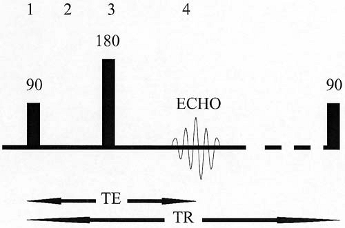 FIG. 1.6. Repetition time (TR) and echo time (TE) for spin echo sequence. TR represents elapsed time between successive 90-degree excitations. TE represents the time delay from the 90-degree excitation to the center of the echo. Note that 180-degree refocusing pulse occurs at time = ½ TE. Large numbers correspond to time points in Figure 1.4, which are notated by the same numbers. |
The time from the center of the excitation pulse to the center of the echo is known as the TE. The refocusing pulse or refocusing gradient occurs halfway between the excitation pulse and the echo (at TE/2). A long TE allows more time for signal loss to occur from T2 decay. Therefore, a long TE allows for substantially greater signal loss from tissues with a short T2 than from tissues with a long T2 (Fig. 1.7). In other words, a long TE allows for differentiation of tissues based on their respective T2 values. Another important point is that a long TE allows more time for the effects of local magnetic field heterogeneities (T2* effects) to occur. As a result, magnetic susceptibility artifacts resulting from metal or air are exaggerated when imaging is performed with a longer TE (Fig. 1.8).
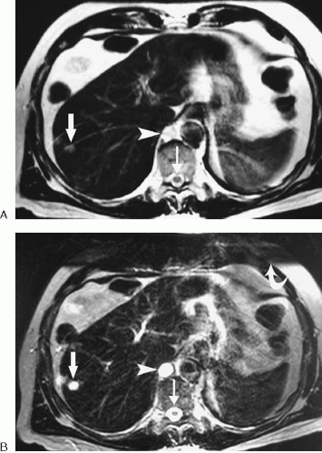 FIG. 1.7. Effect of TE on T2-weighted image. A: TE = 100 msec. Small hemangioma (arrow), cerebrospinal fluid (CSF) (thin arrow), and cisterna chyli (arrowhead) are not significantly different in signal intensity than fat. B: TE = 250 msec. Small hemangioma (arrow), CSF (thin arrow), and cisterna chyli (arrowhead) are significantly more conspicuous due to loss of signal intensity of background tissues having shorter T2. Note the use of a saturation band (curved arrow) over anterior subcutaneous fat to decrease respiratory artifact on this non-breath-hold examination. |
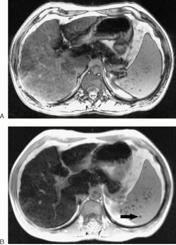 FIG. 1.8. Effect of increasing echo time (TE) in a patient with hemochromatosis. A: Gradient echo T1-weighted image with TE = 2.7 msec. B: Gradient echo T1-weighted image in the same patient with TE = 5.3 msec. Note the lower signal intensity of liver relative to spleen with longer TE due to greater dephasing induced by the presence of parenchymal iron. Siderotic nodules within spleen (arrow) are also more conspicuous. |
Gradients
Producing a signal or echo is only the first step in creating an MR image. Equally important is localizing the signal in space. This may seem an impossible task, because the echo measured in MRI represents signal from the entire volume of tissue excited by the initial RF pulse, and this signal appears graphically like a wavy line. However, the data can be spatially encoded through the use of gradients. As mentioned earlier, a gradient is a linear variation in the magnetic field strength along an axis (although the term gradient is also commonly used to refer to the gradient coils that produce this variation in magnetic field strength). Because the MR signal must be localized in three dimensions, spatial encoding requires the use of three gradients*.
The slice-select gradient is the easiest gradient to understand. To produce signal from only one slice, a gradient is
applied along an axis perpendicular to the desired slice. Because the magnetic field strength varies along this axis, the hydrogen protons precess at different rates based on their location relative to this gradient. A frequency-selective RF pulse (i.e., an RF pulse of a specific frequency) only excites those protons precessing at the same frequency as the RF pulse. Therefore, only protons at a specific location along the gradient are tipped into the transverse plane, and only these protons contribute to the final echo.
applied along an axis perpendicular to the desired slice. Because the magnetic field strength varies along this axis, the hydrogen protons precess at different rates based on their location relative to this gradient. A frequency-selective RF pulse (i.e., an RF pulse of a specific frequency) only excites those protons precessing at the same frequency as the RF pulse. Therefore, only protons at a specific location along the gradient are tipped into the transverse plane, and only these protons contribute to the final echo.
Related posts:
 Scan Optimization: The Art of Compromise
 Magnetic Resonance Urography
 Magnetic Resonance Imaging of the Gastrointestinal Tract
 Modifying Sequence Parameters
 Glossary of Magnetic Resonance Imaging Terms
 What the Surgeon Needs to Know: Preoperative Assessment of Patients with Selected Tumors and Organ Transplant Candidates
Stay updated, free articles. Join our Telegram channel

Full access? Get Clinical Tree


